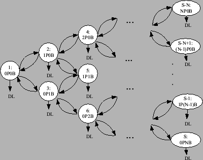
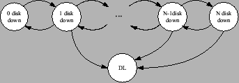
Figure 11 shows the Markov state diagram for
Protocol 1, which can also be applied to the other protocols. In
this diagram, ![]() signifies that the state number/index is
signifies that the state number/index is
![]() , and there are
, and there are ![]() and
and ![]() failed nodes in the primary and
backup group, respectively. All the states shown are working
states, with the exception of
failed nodes in the primary and
backup group, respectively. All the states shown are working
states, with the exception of ![]() , which is the data loss state.
The total number of states in the Markov state diagram is denoted
by
, which is the data loss state.
The total number of states in the Markov state diagram is denoted
by ![]() and is equal to
and is equal to ![]() . The Markov chain begins
with State 1 (
. The Markov chain begins
with State 1 (![]() ), followed by State 2(
), followed by State 2(![]() ), and so on.
), and so on.
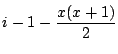
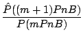
To facilitate the solution to this model, we derive
a function, given in Eqn. 2, that maps from the system state
with ![]() failed primary nodes and
failed primary nodes and ![]() failed backup nodes to
the state index
failed backup nodes to
the state index ![]() of the Markov state diagram:
of the Markov state diagram:
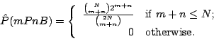
Similarly, the inverse mapping function is given in Eqn. 3
and 4.
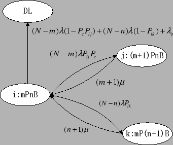
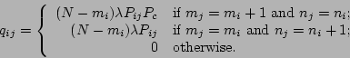
Figure 12 shows the transition rate between the
neighboring states. In the diagram, ![]() denotes the
probability that the system remains functional, also referred to
as safety probability, given that one more primary node
fails while
denotes the
probability that the system remains functional, also referred to
as safety probability, given that one more primary node
fails while ![]() primary nodes and
primary nodes and ![]() backup nodes have already
failed. Similarly,
backup nodes have already
failed. Similarly, ![]() denotes the probability, or safety
probability, of the system remaining functional when one more
backup node fails while
denotes the probability, or safety
probability, of the system remaining functional when one more
backup node fails while ![]() primary nodes and
primary nodes and ![]() backup nodes
have already failed.
backup nodes
have already failed. ![]() can be calculated as
Eqn. 5.
can be calculated as
Eqn. 5.
Similarly, we have
 |
(7) |
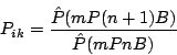
The transition probability from State ![]() to the data loss state,
denoted as
to the data loss state,
denoted as ![]() , can be calculated as Eqn. 8.
, can be calculated as Eqn. 8.
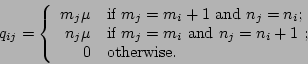
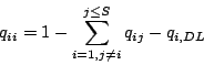
The stochastic transitional probability matrix is defined as
![]() , where
, where
![]() and
and
![]() is the transition probability
from State
is the transition probability
from State ![]() to State
to State ![]() . In summary,
. In summary, ![]() can be calculated as follows.
can be calculated as follows.
If ![]() , then
, then
 |
(9) |
If ![]() , then
, then
 |
(10) |
If ![]() , then
, then
 |
(11) |
If ![]() , i.e., the primary node and backup node are always
kept consistent, like in RAID-1, and a fault-free network is
assumed, the model shown in Figure 11 can be
simplified to the classic RAID-1 model [28], as shown
in Figure 13. This is proven by the fact that
numerical results generated by both models with the same set of
input parameters are identical.
, i.e., the primary node and backup node are always
kept consistent, like in RAID-1, and a fault-free network is
assumed, the model shown in Figure 11 can be
simplified to the classic RAID-1 model [28], as shown
in Figure 13. This is proven by the fact that
numerical results generated by both models with the same set of
input parameters are identical.